Shawn Zhong

Shawn Zhong

钟万祥
  • Tutorials
  • Mathematics
    • Math 240
    • Math 375
    • Math 431
    • Math 514
    • Math 521
    • Math 541
    • Math 632
    • Abstract Algebra
    • Linear Algebra
    • Category Theory
  • Computer Sciences
    • CS/ECE 252
    • CS/ECE 352
    • Learn Haskell
  • AP Notes
    • AP Microecon
    • AP Macroecon
    • AP Statistics
    • AP Chemistry
    • AP Physics E&M
    • AP Physics Mech
    • CLEP Psycho

Home / 2018 / Page 12

Category Theory – Video 4

  • May 23, 2018
  • Shawn
  • Category Theory
  • No comments yet
The Identity Arrow • In S, the Identity Arrow takes each element to itself • e.g. for A={a_0,a_1,a_2 },1_A:A→A≡{█(1_A (a_0 )=a_0@1_A (a_1 )=a_1@1_A (a_2 )=a_2 )┤ • In Music (S), we officially have three more arrows ○ 1_X:X→X ○ 1_Z:Z→Z ○ 1_L:L→L The Identity Laws • Suppose we have a category with objects A and B, then we have 1_A:A→A, 1_B:B→B • The Identity Laws can now be restated to say that, in any Category, this Diagram must Commute • For a diagram to commute, all paths between two objects must be interpreted as the same arrow • Example ○ Suppose f(a_0 )=b_0, then ○ (f∘1_A )(a_0 )=f(1_A (a_0 ))=f(a_0 )=b_0 ○ (1_B∘f)(a_0 )=1_B (f(a_0 ))=1_B (b_0 )=b_0 The Category of Sets With an Endomorphism S^↺ • A^(↺1_A ) and B^(↺1_B ) are objects in S^↺, but what shoud the arrows be? • We want every f:A→B in S to be an arrow f:A^(↺1_A )→B^(↺1_B ) in S^↺ • The law f must follow in S: f∘1_A=1_B∘f, can we generalize this? • What if we replaced 1_A with any endomorphism α, and 1_B with β • Then we get a map f:A^(↺1_A )→B^(↺1_B ) in S^↺ that satisfy: f∘α=β∘f The Associative Law • We have four objects, A,B,C, and D, with arrows f:A→B, g:B→C, and h:C→D • The associativity law says that this diagram must commute • We have 3 paths A→D. They are h∘(g∘f),(hg)∘f, and h∘g∘f • They all must be interpreted as the same map A→D • Example ○ A={a_0,a_1 }, B={b_0,b_1,b_2 }, C={c_0,c_1 },D={d_0,d_1,d_2 } ○ f:A→B≡{█(f(a_0 )=b_0@f(a_1 )=b_1 )┤ ○ g:B→C≡{█(g(b_0 )=g(b_2 )=c_1@g(b_1 )=c_0 )┤ ○ h:C→D≡h(c_0 )=h(c_1 )=d_1
Read More >>

Category Theory – Video 5

  • May 23, 2018
  • Shawn
  • Category Theory
  • No comments yet
Calculating The Number of Maps Between Sets • Consider A={a_0,a_1 }, B={b_0,b_1,b_2 } • There are 3×3=9 maps from A to B • There are 2×2×2=8 maps from B to A General Formula for The Number of Maps A→B • In general, the number of maps A→B is |B|^|A| because each a_i has |B| independent choices • The number of maps A→B≡|B^A |=|B|^|A| • In Video 2, we have defined ○ X={x_0,x_1,x_2,x_3,x_4,x_5,x_6,x_7,x_8,x_9,x_10,x_11 } ○ C={C♮,(C♯/D♭),D♮,(D♯\/E♭),E♮,F♮,(F♯/G♭),G♮,(G♯/A♭),A♮,(A♯\/B♭),B♮} • So |X^C |=|〖12〗^12 |=8,916,100,448,256 Universal Mapping Properties (UMPs) • A Universal Mapping Property asserts something about one or more objects with zero or more maps between them in relation to all other objects X in the Category • A UMP is an object P, that may or may not have a relationship to a diagram of some sort • The principal is that there is only one map between P and all other objects X in that Category • With X as either the Domain or Codomain of that map, such that P still obeys its restriction Initial Object • In any Category C, an object 0 is said to be an Initial Object of C, if ∀X in C, there is a unique C-arrow 0→X • In S, a set 0 is said to be an Initial Object of S, if for all sets X, there is a unique map 0→X • Number of maps A→B is represented by |B^A |=|B|^|A| , so |X|^|0| =1 must hold for all X • So the Initial Set is the Empty Set, because any number raised to the power of 0 is 1 • There are no maps X→0, unless X≅0, since 0 raised to the power of any number (except 0) is 0 Duality • Whenever you define a UMP in S, to get another UMP just "do the opposite of what the definition says" • Usually just by reversing the arrows, and you ll get another UMP for free • Just add the prefix "co-" to the original definition and you’re done Terminal Object • In any Category C, an object T is said to be a Terminal Object of C, if ∀X in C, there is a unique C-arrow X→T • In S, a set T is said to be a Terminal Object of S, if for all sets X, there is a unique map X→T • Number of maps A→B is represented by |B^A |=|B|^|A| , so |T|^|X| =1 must hold for all X • The Terminal Set is 1, because 1 raised to the power of any number is 1 The Opposite Category and Duality • Duality ○ What if for every map f:A→B, we define a map f^op:B→A that makes the same associations between A and B, just from B^′ s perspective? ○ The map f^op:B→A assigns to each b_i∈B a subset A_i of A called the Splitting of b_i, defined as {a∈A_i⇔f^op (b_i )=a}, such that for all a∈A, there is exactly one A_i such that a∈A_i • Opposite Category ○ We can form a new category S^op that is the "mirror", or Opposite Category of S ○ For every object in S, there is a correspondent object in S^op ○ For every arrow f:A→B in S, there is a correspondent arrow f^op:B→A in S^op Calculating the Number of Maps 3→2 in S^op • The number of maps 3→2 in S^op must be 9, because there are 9 maps 2→3 in S • Ideally each element of the Domain in S^op has 3 choices in a map into the Codomain 2 ○ 0: Do nothing ○ 1: Connect ○ 2: Split into 2 • If we want to partition 2 into 3 parts, our options are 2+0+0, and 1+1+0 • We will represent the size of the subset that f^op assigns to b_0,b_1,b_2 as ⟨|A_0 |,|A_1 |,|A_2 |⟩ The Terminal Object in S^op • The Terminal Object in S^op is the Initial Object in S • The Initial Object in S^op is the Terminal Object in S
Read More >>

Category Theory – Video 6

  • May 23, 2018
  • Shawn
  • Category Theory
  • No comments yet
Read More >>

Deploy WordPress on CS Lab Server

  • Apr 24, 2018
  • Shawn
  • Tutorials
  • No comments yet
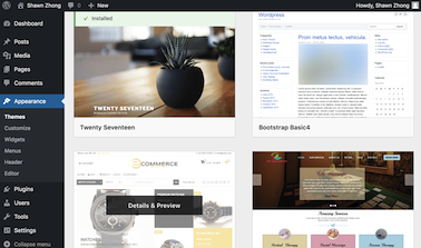
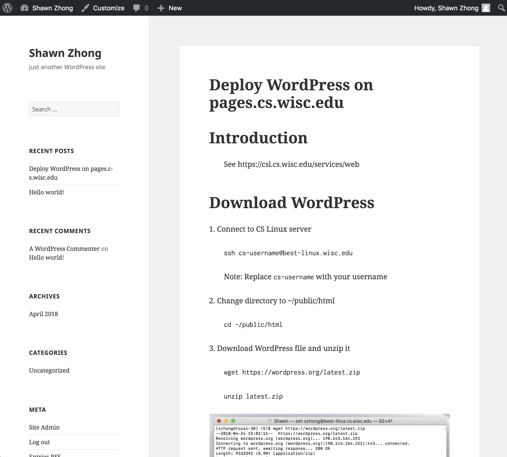
This tutorial walks through how you can deploy WordPress on a CS Department Server. (more…)
Read More >>

11.1 Introduction to Trees

  • May 07, 2018
  • Shawn
  • Math 240
  • No comments yet
Trees • Definition ○ A tree is a connected undirected graph with no simple circuits. • Example ○ Which of these graphs are trees? • Solution ○ G_1 and G_2 are trees - both are connected and have no simple circuits ○ Because e, b, a, d, e is a simple circuit, G_3 is not a tree. ○ G_4 is not a tree because it is not connected. • Definition ○ A forest is a graph that has no simple circuit, but is not connected. ○ Each of the connected components in a forest is a tree. • Theorem ○ An undirected graph is a tree if and only if there is a unique simple path between any two of its vertices. • Proof ○ (⟹)Assume that T is a tree. § Then T is connected with no simple circuits. § Hence, if x and y are distinct vertices of T, there is a simple path between them (by Theorem 1 of Section 10.4). § This path must be unique - for if there were a second path, there would be a simple circuit in T (by Exercise 59 of Section 10.4). § Hence, there is a unique simple path between any two vertices of a tree. ○ (⟸)Now assume that there is a unique simple path between any two vertices of a graph T. § Then T is connected because there is a path between any two of its vertices. § Furthermore, T can have no simple circuits since if there were a simple circuit, there would be two paths between some two vertices. ○ Hence, a graph with a unique simple path between any two vertices is a tree. Rooted Trees • Definition ○ A rooted tree is a tree in which one vertex has been designated as the root and every edge is directed away from the root. • An unrooted tree is converted into different rooted trees when different vertices are chosen as the root. Rooted Tree Terminology • Terminology for rooted trees is a mix from botany and genealogy (such as this family tree of the Bernoulli family of mathematicians). • If v is a vertex of a rooted tree other than the root, the parent of v is the unique vertex u such that there is a directed edge from u to v. • When u is a parent of v, v is called a child of u. • Vertices with the same parent are called siblings. • The ancestors of a vertex are the vertices in the path from the root to this vertex, excluding the vertex itself and including the root. • The descendants of a vertex v are those vertices that have v as an ancestor. • A vertex of a rooted tree with no children is called a leaf. • Vertices that have children are called internal vertices. • If a is a vertex in a tree, the subtree with a as its root is the subgraph of the tree consisting of a and its descendants and all edges incident to these descendants. Examples of Rooted Trees • Example: In the rooted tree T (with root a): ○ Find the parent of c, the children of g, the siblings of h, the ancestors of e, and the descendants of b. ○ Find all internal vertices and all leaves. ○ What is the subtree rooted at G? • Solution: ○ The parent of c is b. The children of g are h, i, and j. The siblings of h are i and j. The ancestors of e are c, b, and a. The descendants of b are c, d, and e. ○ The internal vertices are a, b, c, g, h, and j. The leaves are d, e, f, i, k, l, and m. ○ We display the subtree rooted at g. Properties of Trees • Theorem 2 ○ A tree with n vertices has n − 1 edges. • Proof (by mathematical induction): ○ Basis Step § When n = 1, a tree with one vertex has no edges. § Hence, the theorem holds when n = 1. ○ Inductive Step § Assume that every tree with k vertices has k − 1 edges. § Suppose that a tree T has k + 1 vertices and that v is a leaf of T. § Let w be the parent of v. § Removing the vertex v and the edge connecting w to v produces a tree T′ with k vertices. § By the inductive hypothesis, T′ has k − 1 edges. § Because T has one more edge than T′, we see that T has k edges. § This completes the inductive step. m-ary Rooted Trees • Definition ○ A rooted tree is called an m-ary tree if every internal vertex has no more than m children. ○ The tree is called a full m-ary tree if every internal vertex has exactly m children. ○ An m-ary tree with m = 2 is called a binary tree. • Example ○ Are the following rooted trees full m-ary trees for some positive integer m? • Solution ○ T_1 is a full binary tree because each of its internal vertices has two children. ○ T_2 is a full 3-ary tree because each of its internal vertices has three children. ○ In T_3 each internal vertex has five children, so T3 is a full 5-ary tree. ○ T_4 is not a full m-ary tree for any m because some of its internal vertices have two children and others have three children. Counting Vertices in Full m-Ary Trees • Theorem 3 ○ A full m-ary tree with i internal vertices has n = mi + 1 vertices. • Proof ○ Every vertex, except the root, is the child of an internal vertex. ○ Because each of the i internal vertices has m children, ○ there are mi vertices in the tree other than the root. ○ Hence, the tree contains n = mi + 1 vertices. • Theorem 4 ○ A full m-ary tree with § n vertices has i=(n−1)/m internal vertices and l=((m−1)n+1)/m leaves, § i internal vertices has n = mi + 1 vertices and l=(m−1)i+1 leaves, § l leaves has n=(ml−1)/(m−1) vertices and i=(l−1)/(m−1) internal vertices. ○ Proof (of part i) § Solving for i in n = mi + 1 (from Theorem 3) gives i=(n−1)/m. § Since each vertex is either a leaf or an internal vertex, n=l+i. § By solving for l and using the formula for i, we see that § l=n−i=n−(n−1)/m=((m−1)n+1)/m Level of vertices and height of trees • When working with trees, we often want to have rooted trees where the subtrees at each vertex contain paths of approximately the same length. • To make this idea precise we need some definitions: ○ The level of a vertex v in a rooted tree is the length of the unique path from the root to this vertex. ○ The height of a rooted tree is the maximum of the levels of the vertices. • Example: ○ Find the level of each vertex in the tree to the right. ○ What is the height of the tree? • Solution: ○ The root a is at level 0. ○ Vertices b, j, and k are at level 1. ○ Vertices c, e, f, and l are at level 2. ○ Vertices d, g, i, m, and n are at level 3. ○ Vertex h is at level 4. ○ The height is 4, since 4 is the largest level of any vertex. Balanced m-Ary Trees • Definition ○ A rooted m-ary tree of height h is balanced if all leaves are at levels h or h − 1. • Example ○ Which of the rooted trees shown below is balanced? • Solution ○ T_1 and T_3 are balanced, but T_2 is not because it has leaves at levels 2, 3, and 4. The Bound for the Number of Leaves in an m-Ary Tree • Theorem 5 ○ There are at most mh leaves in an m-ary tree of height h. • Proof (by mathematical induction on height): ○ Basis Step § Consider an m-ary trees of height 1. § The tree consists of a root and no more than m children, all leaves. § Hence, there are no more than m^1=m leaves in an m-ary tree of height 1. ○ Inductive Step § Assume the result is true for all m-ary trees of height   h. § Let T be an m-ary tree of height h. § The leaves of T are the leaves of the subtrees of T we get when we delete the edges from the root to each of the vertices of level 1. § Each of these subtrees has height ≤ h−1. § By the inductive hypothesis, each of these subtrees has at most mh− 1 leaves. § Since there are at most m such subtrees, there are at most m⋅m^(h1) = mh leaves in the tree. • Corollary 1 ○ If an m-ary tree of height h has l leaves, then h ≥ ⌈log_m⁡l⌉. ○ If the m-ary tree is full and balanced, then h = ⌈log_m⁡l⌉. (see text for the proof)
Read More >>
  • 1
  • …
  • 10
  • 11
  • 12
  • 13
  • 14
  • …
  • 41

Search

  • Home Page
  • Tutorials
  • Mathematics
    • Math 240 – Discrete Math
    • Math 375 – Linear Algebra
    • Math 431 – Intro to Probability
    • Math 514 – Numerical Analysis
    • Math 521 – Analysis I
    • Math 541 – Abstract Algebra
    • Math 632 – Stochastic Processes
    • Abstract Algebra @ 万门大学
    • Linear Algebra @ 万门大学
    • Category Theory
  • Computer Sciences
    • CS/ECE 252 – Intro to Computer Engr.
    • CS/ECE 352 – Digital System Fund.
    • Learn Haskell
  • Course Notes
    • AP Macroeconomics
    • AP Microeconomics
    • AP Chemistry
    • AP Statistics
    • AP Physics C: E&M
    • AP Physics C: Mechanics
    • CLEP Psychology
  • 2048 Game
  • HiMCM 2016
  • 登峰杯 MCM

WeChat Account

Categories

  • Notes (418)
    • AP (115)
      • AP Macroeconomics (20)
      • AP Microeconomics (23)
      • AP Physics C E&M (25)
      • AP Physics C Mechanics (28)
      • AP Statistics (19)
    • Computer Sciences (2)
    • Mathematics (300)
      • Abstract Algebra (29)
      • Category Theory (7)
      • Linear Algebra (29)
      • Math 240 (42)
      • Math 375 (71)
      • Math 514 (18)
      • Math 521 (39)
      • Math 541 (39)
      • Math 632 (26)
  • Projects (2)
  • Tutorials (11)

Archives

  • October 2019
  • May 2019
  • April 2019
  • March 2019
  • February 2019
  • December 2018
  • November 2018
  • October 2018
  • September 2018
  • July 2018
  • May 2018
  • April 2018
  • March 2018
  • February 2018
  • January 2018
  • December 2017
  • November 2017
  • October 2017
  • September 2017
  • August 2017
  • July 2017
  • June 2017

WeChat Account

Links

RobeZH's thoughts on Algorithms - Ziyi Zhang
Copyright © 2018.      
TOP